This example can be developed on the blackboard for 10 to 15 minutes.
Example: Fourier $d_n$ coefficients of an asymmetrical square pulse train
Problem Statement
Find the coefficients for the Fourier series of the signal $f(t)$
Approach
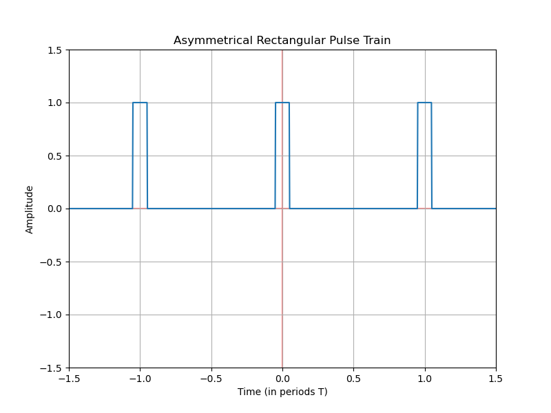
Pulse Train
The signal is a pulse train, as in previous example, but in this case, the pulse occupies one-fifth of the train; or in other words, one-tenth of the period.
Generating Function
\begin{equation} f(t) = \pi \left( \frac{t-nT}{T/10}\right) \end{equation}
Spectrum
For this example, finding the coefficients for the Fourier serier of the signal $d_n$ will be equivalent to represent the spectrum of the signal.
Solution
By only varying the integration limits, we can follow the calculations from the first example, where the description of the steps can be read.
\[\begin{aligned} d_n &= \frac{1}{T} \int_{-\infty}^{\infty} f(t) e^{-j 2\pi n f_0 t} \, dt \\ &= \frac{1}{T} \int_{-T/20}^{T/20} \pi \left( \frac{t}{T/2} \right) e^{-j 2\pi n f_0 t} \, dt \\ &= \frac{1}{T} \cdot \frac{-1}{j 2\pi n f_0} \left[ e^{-j 2 \pi n f_0 t} \right]_{-T/20}^{T/20} \\ &= \frac{1}{T} \cdot \frac{-1}{j 2\pi n f_0} \left[ e^{\frac{-j 2 \pi n f_0 T}{10}} - e^{\frac{+j 2 \pi n f_0 T}{4}} \right] \\ &= \frac{e^{\frac{j \pi n}{10}} - e^{\frac{-j \pi n}{10}}}{j 2\pi n} \\ &= \frac{\cos\left(\frac{\pi n}{10}\right) + j \sin\left(\frac{\pi n}{10}\right) - \cos\left(\frac{-\pi n}{10}\right) - j \sin\left(\frac{-\pi n}{10}\right)}{j 2\pi n} \\ &= \frac{\cos\left(\frac{\pi n}{10}\right) + j \sin\left(\frac{\pi n}{10}\right) - \cos\left(\frac{\pi n}{10}\right) + j \sin\left(\frac{\pi n}{10}\right)}{j 2\pi n} \\ &= \frac{j 2 \sin\left(\frac{\pi n}{10}\right)}{j 2\pi n} = \frac{\sin\left(\frac{\pi n}{10}\right)}{\pi n} = \frac{1}{10} \frac{\sin\left(\frac{\pi n}{10}\right)}{\frac{\pi n}{10}} = \frac{1}{10} sinc_n\left(\frac{n}{10}\right) \end{aligned}\]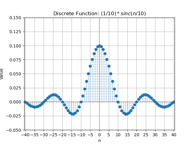
Conclussions
Spectrum Morphology
The amplitude spectrum in the last figure although with a lower level (the maximum amplitude value is 0.1), logically has the same shape as the corresponding pulse train with the same high and low duration; however, the density of spectral lines has increased. The width of the main lobe has also increased, which could mean that if a single harmonic was enough to reconstruct the wide pulse with good approximation, 10 harmonics would be needed to reconstruct the narrow pulse.
Bandiwdth
Narrow pulses require more \textbf{bandwidth} to be reconstructed. An amplifier for \textit{fast} signals requires greater bandwidth than an amplifier for \textit{slow} signals, even if they are signals of the same frequency.
Limit case $T \simeq \infty$
If $T$ increases to become infinite, which would be equivalent to a signal with a single pulse, then the spectrum density would increase until it becomes continuous.