This example can be developed on the blackboard for 20 to 30 minutes, if followed by a previous exmample.
Example: Fourier series of a symmetrical bipolar square pulse train
Problem Statement
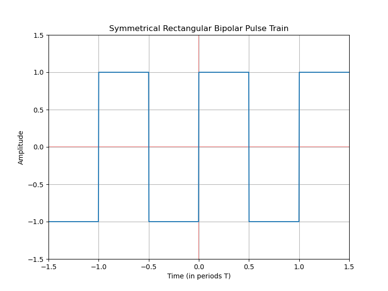
Develop the Fourier series of the signal $g(t)$
Approach
Periodic Alternating Function
The function is periodic; the value alternates between 1 and -1.
Choice of Period
The function resembles a sine wave centered at 0. The period starts at 1 and ends at -1. We choose the period from $-T/2$ to $T/2$, which is centered at the origin. This will facilitate the integration of the function within this period.
Generating Function
It consists of two pulses, each with a width of $T/2$ and offset, one at $-T/4$ and the other at $T/4$: \begin{equation} g(t)=-\pi \left(\frac{t+\frac{T}{4}}{\frac{T}{2}} \right) + \pi \left( \frac{t-\frac{T}{4}}{\frac{T}{2}} \right) \end{equation}
Solution
Coefficients $d_n$
To obtain a Fourier series, the coefficients $d_n$ must first be calculated: \begin{equation} d_n=\frac{1}{T} \int_{-\infty}^{\infty} f(t) e^{-j 2\pi n f_0 t} d t \end{equation}
Periodic Function
We integrate the generating function over one period, choosing a period $T$ centered at the origin: \begin{equation} d_n=\frac{1}{T} \int_{-T/2}^{0} -\pi \left(\frac{t+\frac{T}{4}}{\frac{T}{2}} \right) e^{-j 2\pi n f_0 t} d t + \frac{1}{T} \int_{0}^{T/2} \pi \left( \frac{t-\frac{T}{4}}{\frac{T}{2}} \right) e^{-j 2\pi n f_0 t} d t \end{equation}
Simplify the Integration Limits
The periodic function is 1, 0, or -1; we integrate over the limits where it is 1 or -1: \begin{equation} d_n=\frac{-1}{T} \int_{-T/2}^{0} e^{-j 2\pi n f_0 t} d t + \frac{1}{T} \int_{0}^{T/2} e^{-j 2\pi n f_0 t} d t \end{equation}
Integrate
\begin{equation} d_n = \frac{-1}{T} \frac {-1}{j 2 \pi n f_0} \left[ e^{-j 2 \pi n f_0 t}\right]_{-T/2}^0 + \frac{1}{T} \frac {-1}{j 2 \pi n f_0} \left[ e^{-j 2 \pi n f_0 t}\right]_0^{T/2} \end{equation}
\begin{equation} d_n= \frac{1}{j 2 \pi n f_0 T} \left( \left[ e^{-j 2 \pi n f_0 t}\right] _{-T/2}^0 - \left[ e^{-j 2 \pi n f_0 t}\right] _0^{T/2} \right) \end{equation}
\begin{equation} d_n= \frac{1}{j 2 \pi n \cancel{f_0 T}} \left( 1 - e^{j \cancel{2} \pi n \cancel{f_0} \frac {\cancel{T}}{\cancel{2}}} - e^{-j \cancel{2} \pi n \cancel{f_0} \frac{\cancel{T}}{\cancel{2}}} +1 \right) \end{equation} \begin{equation} d_n= \frac{1}{j 2 \pi n } \left( - e^{j \pi n } - e^{-j \pi n } +2 \right) \end{equation} \begin{equation} d_na = \frac{1}{j \pi n } \left(-\frac { e^{j \pi n } + e^{-j \pi n }}{2} +1 \right) \end{equation} \begin{equation} d_n= \frac{1}{j \pi n } \left(-\cos \left( \pi n \right) +1 \right) \end{equation}
Sine
Using the trigonometric identity, we get the expression in sine form: \begin{equation} d_n = \frac{2}{j \pi n } \left(\frac{1}{2}-\frac{1}{2}\cos \left( \pi n \right) \right)= \frac{2}{j \pi n } \sin^2\left( \frac{\pi n}{2}\right)
\end{equation}
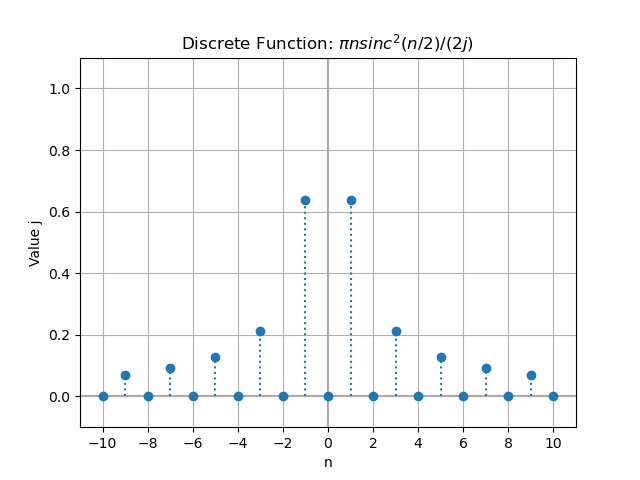
Sinc Function
Expressed in terms of the sinc function: \begin{equation} d_n = \frac{\pi n}{j 2} \frac{\sin^2\left( \frac{\pi n}{2}\right)}{\left(\frac{\pi n}{2}\right)^2}= \frac{\pi n}{j 2} sinc^2\left( \frac{\pi n}{2} \right) = \frac{\pi n}{j 2} sinc_n^2\left( \frac{n}{2} \right) \end{equation}
Fourier Series
Substituting into the Fourier transform expression:
\begin{align} f(t) &= \sum_{n=-\infty}^\infty d_n e^{j 2 \pi n f_0 n t} = \sum_{n=-\infty}^\infty \frac{\pi n}{j 2} sinc_n^2\left( \frac{n}{2} \right) e^{j 2 \pi n f_0 n t}
&= \frac{\pi}{j 2} \sum_{n=-\infty}^\infty n sinc_n^2\left( \frac{n}{2} \right) \left[\cos\left( 2 \pi n f_0 t \right)+j\sin\left( 2 \pi n f_0 t \right) \right] \ &= \frac{\pi}{j 2} \left[\sum_{n=-\infty}^\infty n sinc_n^2\left( \frac{n}{2} \right)\cos\left( 2 \pi n f_0 t \right)+ \sum_{n=-\infty}^\infty n sinc_n^2\left( \frac{n}{2} \right) j\sin\left( 2 \pi n f_0 t \right) \right] \end{align}
Summation and Integral
The summation operation for a discrete function is equivalent to the integration operation for a continuous function; the properties of even and odd functions in integration are the same as in summation.
Odd Function
The product of the functions $n$ (odd), $sinc^2(\frac{n}{2})$ (even), and $\cos(2 \pi n f_0 t)$ (even) is odd. Therefore, the summation over $\mathbb{N}$ is $0$. \begin{equation} f(t)= \frac{\pi}{\cancel{j} 2} \sum_{n=-\infty}^\infty n sinc_n^2\left( \frac{n}{2} \right) \cancel{j}\sin\left( 2 \pi n f_0 t \right) \end{equation}
Even Function
The product of the functions $n$ (odd), $sinc^2(\frac{n}{2})$ (even), and $\sin(2 \pi n f_0 t)$ (odd) is even. Therefore, the summation can be rewritten as: \begin{equation} f(t)= \frac{\cancel{2} \pi}{ \cancel{2}} \sum_{n=0}^\infty n sinc_n^2\left( \frac{n}{2} \right) \sin\left( 2 \pi n f_0 t \right) = \pi\sum_{n=1}^\infty n sinc_n^2\left( \frac{n}{2} \right) \sin\left( 2 \pi n f_0 t \right) \end{equation}
Series Values
We tabulate some values of the series:
| $n$ | $n \pi sinc_n^2 \left( \frac{n}{2} \right)$ | $\sin\left( 2 \pi n f_0 t \right)$ |
|---|---|---|
| 0 | 1 | 0 |
| 1 | $\frac{4}{\pi}$ | $\sin(2 \pi f_0 t)$ |
| 2 | 0 | $\sin(4 \pi f_0 t)$ |
| 3 | $\frac{4}{3 \pi}$ | $\sin(6 \pi f_0 t)$ |
| 4 | 0 | $\sin(8 \pi f_0 t)$ |
| 5 | $\frac{4}{5 \pi}$ | $\sin(10 \pi f_0 t)$ |
| 6 | 0 | $\sin(12 \pi f_0 t)$ |
| 7 | $\frac{4}{7 \pi}$ | $\sin(14 \pi f_0 t)$ |
Summation
It can also be written in a more compact form:
\begin{equation} f(t) = \frac{4}{\pi} \sum_1^{\infty} \frac{1}{2n-1}\sin \left(2 (2n-1) \pi f_0 t \right) \end{equation}
Graphical Representation
When we superimpose the original signal on the terms of the obtained series, we see that the series increasingly resembles the signal as more terms are added. 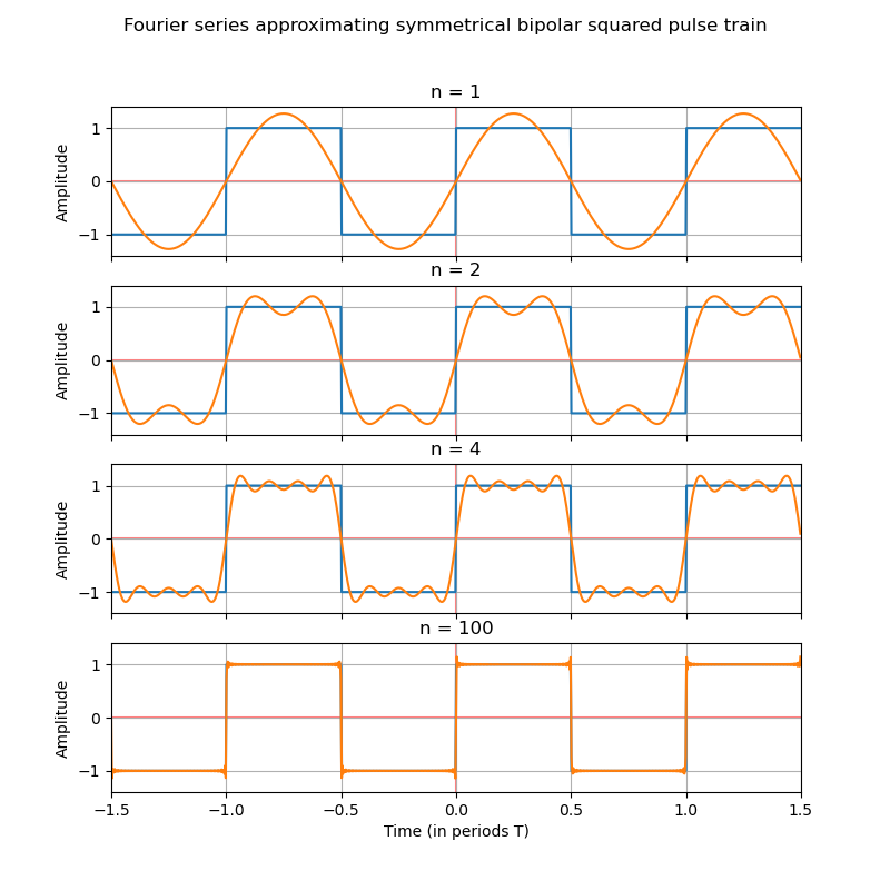 As we add terms to the series, it increasingly resembles the original signal.
Conclussions
Parity of a function
The signal in the previous example (pair) was built upon a Fourier Series made up of fundamental cosinus functions. This (odd), besides similary, is build up by fundamental sinus functions.
Mean value of a function
In contrast to the previous example where the signal was not centered at zero, resulting in a non-zero first frequency component (which was the average amplitude of the signal), the current signal is centered at zero. Consequently, the first frequency component is zero. This centering of the signal simplifies the analysis and ensures that the DC component is null, emphasizing the symmetrical nature of the signal around the origin. Additionally, the Fourier series representation highlights the importance of symmetry in simplifying the frequency domain analysis, demonstrating that signals centered at zero tend to have more straightforward Fourier series with zero DC components. This property is particularly useful in applications where the elimination of the DC offset is desirable for signal processing tasks.